In this second blog post I am following up on last week's introduction to category theory, and I am covering a particular kind of category equipped with extra data called a monoidal category. I've already spoiled a great deal about these monoidal categories in my last post, where I've mentioned the reason that they are interesting is that they admit a diagrammatic language, and thus we can reason about them by drawing pictures. In this post I hope to describe the structure of a monoidal category in more abstract terms, as well as introduce the graphical calculus. The idea is that this extra data which makes a category into a monoidal category works to describe how morphisms can be composed in parallel, and thus pictures can much better represent parallel compositions due to the fact that we can make use of the 2D plane and write morphisms “side by side ”. Furthermore, if we admit non-trivial braiding of morphisms, the dimension needed to represent the graphical calculus goes up to three, since as we will see we can bend “wires ” around each other in 3D space. Note that this post is simply a slightly digested (but mostly faithful to the original) version of Chapter 1 of “Categories for Quantum Theory ” by Heunen and Vicary. In these notes, the fact that this blog is merely a glorified note-taking project becomes clear :-). Refer to the original book for a better description of basically everything I am writing here.
The structure of a Monoidal category (algebraically)
The most natural way to interpret a category is that systems are objects, and morphisms are processes which change said objects, or turn some objects into others. This idea is at the root of the “process ” interpretation of quantum mechanics, underlying Bob Coecke's and Alex Kissinger 's beautiful book “Picturing Quantum Processes ”, where categorical quantum mechanics is explained very pedagogically. As I stated in last week's post, the idea of categories is to allow composition of these processes, i.e. morphisms are composed “vertically ” in the page, whereas the idea of monoidal categories is that we can also let processes happen “simultaneously ”, or “in parallel ”.
So, a new symbol is necessary to express this parallel composition. The symbol \(\otimes\) is used most often, and is generically called a “tensor product ” or sometimes simply “tensor ”. One of the key aspects of monoidal categories is that unlike what us physicists are used, in assuming that \(\left(A\otimes B\right)\otimes C\) and \(A\otimes\left(B\otimes C\right)\) are equal, for monoidal categories this is not always true. Indeed, this is often too strong of an assumption, even for the applications of monoidal categories to physical theories. I will hopefully, some day in the future, give the example of anyons, where the “fusion rules ”, i.e. the tensor product structure is different depending of the order of “fusion ”, and instead the relation between different orders of fusion is encoded in the so-called \(F-\)matrices. Generically, a monoidal category is defined as
Definition (Monoidal category):
A monoidal category is a category \(\boldsymbol{C}\) equipped with the following data:
- A tensor product functor \(\otimes:\boldsymbol{C}\times\boldsymbol{C}\to\boldsymbol{C}\)
- A unit object \(I\in\text{Ob}(\boldsymbol{C})\)
- An natural isomorphism called the associator \(\left(A\otimes B\right)\otimes C\overset{\alpha_{A,B,C}}{\longrightarrow}A\otimes\left(B\otimes C\right)\)
- A natural isomorphism called the left unitor \(I\otimes A\overset{\lambda_{A}}{\longrightarrow}A\)
- A natural isomorphism called the right unitor \(A\otimes I\overset{\rho_{A}}{\longrightarrow}A\)
Recall \(\lambda\) naturally stands for left and \(\rho\) for right. The point here is that objects are related by natural isomorphisms, and are not required to be straight up equal. This distinction seems pathological, and so does the distinction between left and right unitors. That's the annoying price one pays for generality: One has to deal with distinctions between left and right, distinctions between natural isomorphisms and equalities, etc. But as I have previously stated, these seemingly pedantic differences actually prove to be very relevant, even in the context of physics.
Now, to ensure the proper behavior of the associators and unitors, a monoidal category is required to satisfy additional axioms, which are called the triangle and pentagon equations. These requirements are best stated in terms of commutative diagrams
Additionally, since we are imposing that \(\alpha,\lambda\) and \(\rho\) are natural transformations, then we have the following equations
Now, a brief word on the role of these equations is in order. Firstly, the unit object \(I\) is to be interpreted as the “empty ” object. It being or not being there makes absolutely no difference. The unitors establish the isomorphism of both \(I\otimes A\) and \(A\otimes I\) to \(A\). This means that either of these composite objects is just as good as \(A\).
The triangle and pentagon equations establish the coherence of the unitors and associators, stating that two ways of reorganizing a system are equal. This, in turn, implies that any two such reorganizations are equal, which is the content of MacLane's coherence theorem.
Theorem (MacLane's coherence theorem for monoidal categories):
Given the data of a monoidal category, if the triangle and pentagon equations hold, any equation built from \(\alpha,\lambda,\rho\) and their inverses holds.
Together, these equations also imply \(\rho_{I}=\lambda_{I}\), and thus, there is actually no distinction between left and right unitors for the unit object itself.
So, in summary, while the associators and unitors are non-trivial morphisms, satisfying coherence implies that the tensor product obeys all the familiar properties it should, since the way we apply them does not actually matter in any particular case.
Another theorem relates the parallel and sequential compositions:
Theorem (Interchange):
Given four morphisms \(f:A\to B,g:B\to C\) and \(h:D\to E,j:E\to F\) in a monoidal category, they satisfy the interchange law
\[\left(g\circ f\right)\otimes\left(j\circ h\right)=\left(g\otimes j\right)\circ\left(f\otimes h\right)\]
The proof is simple enough that we can give it here as an example. We merely use the definition of the tensor product functor, followed by the composition in \(\boldsymbol{C}\times\boldsymbol{C}\) and functoriality of the tensor product \(\otimes\):
\[\begin{align*} \left(g\circ f\right)\otimes\left(j\circ h\right) & \equiv\otimes\left(g\circ f,j\circ h\right)\\ & =\otimes\left(\left(g,j\right)\circ\left(f,h\right)\right)\\ & =\left(\otimes\left(g,j\right)\right)\circ\left(\otimes\left(f,h\right)\right)\\ & =\left(g\otimes j\right)\circ\left(f\otimes h\right). \end{align*}\] This concludes the proof.
The graphical calculus
In the last section, we described how the setting of monoidal categories, and the definition of the tensor product \(\otimes\) allows us to compose processes in parallel. For morphisms \(f:A\to B\) and \(g:C\to D\), we can draw their parallel composition as
The graphical calculus for monoidal categories is planar, and vertical compositi on, as in the previous blog post represents \(\circ\), while horizontal juxtaposition represents \(\otimes\). Remarkably, this diagrammatic language is not informal, but rather, is said to be both complete and sound. Completeness means that every equation which can be typed for monoidal categories can be written in terms of diagrams, while soundness means that equality of diagrams implies equality of the corresponding typed equations and vice-versa.
Furthermore, the unit object \(I\) is drawn as the empty diagram, i.e. not drawn, and therefore, the associators are also simply not drawn. Here, we write the interchange theorem given in the previous section by artificially drawing some brackets in the diagram representing sequential and parallel composition of morphisms \(f:A\to B,g:B\to C\) and \(h:D\to E,j:E\to F\).
The brackets merely indicate the interpretation we give to the diagram, but removing them makes it clear that the graphical notation makes these identities fairly trivial simply by looking at the diagrams. Thus, this graphical notation makes the seemingly complex aspects of monoidal categories melt away: Unitors, associators, the triangle and pentagon equations , the interchange theorem, and other superficial aspects are absorbed into the drawings themselves.
Furthermore, by planar isotopic deformation of the graphical calculus, one can correctly represent well typed equations in a monoidal category. This can be stated as a theorem
Theorem (Correctness of the graphical calculus for monoidal categories):
A well-typed equation between morphisms in a monoidal category follows from the axioms if and only if it holds in the graphical language up to planar isotopy.
This mention of planar isotopy basically means “up to deformations ” within some rectangular region of the plane, with “input ” wires terminating at the bottom of the rectangle, and “output ” wires terminating at the top. For instance, boxes without inputs can be moved around so long as they do not cross wires:
This correctness theorem states that, like the graphical calculus for the generic graphical calculus of categories, in the setting of monoidal categories , this graphical calculus of monoidal categories, is both sound and complete. I will not delve deeper into these notions here, focusing now on a special type of boxes which can occur in the graphical calculus, for “deleting ” and “co-deleting ” morphisms. In the context of categorical quantum mechanics, these are often called “effects ” and “states ”.
Definition (State and effect):
In a monoidal category, a state of an object \(A\) is simply a morphism \(a:I\to A\). An effect of an object \(A\) is the dual notion, consisting of a morphism \(\overline{a}:A\to I\).
States and effects can be represented by triangles in the graphical notation.
It may be the case that to specify an equality of morphisms, one merely has to check how they affect states, and this motivates the notion of a “well-pointed monoidal category ”.
Definition (Well-pointed, and monoidally well pointed monoidal categories):
A monoidal category is well-pointed if for all parallel pairs of morphisms \(f,g:A\to B\), then \(f=g\) if and only if \(f\circ a=g\circ a\), for all states \(a:I\to A\). If it is the case that for all parallel pairs of morphisms \(f,g:A_{1}\otimes A_{2}\otimes\cdots\otimes A_{n}\to B\), and all states \(a_{1},a_{2},\dots,a_{n}:I\to A\), \(f=g\) if and only if \(f\circ\left(a_{1}\otimes a_{2}\otimes\cdots\otimes a_{n}\right)=g\circ\left(a_{1}\otimes a_{2}\otimes\cdots\otimes a_{n}\right)\), then the category is called monoidally well pointed.
The notion of monoidally well pointed is merely the generalization of well pointed for parallel states. Now, the fascinating thing is that we can construct familiar notions of product states and entangled states in this setting of category theory, without referencing Hilbert spaces at all. Note, that in a monoidal category we can have a morphism \(c:I\to A\otimes B\). Such a morphism is called a joint state of objects \(A\) and \(B\).
Definition (Product state):
A product state is a joint state \(c:I\to A\) when it is of the form \(a\otimes b\circ\lambda_{I}^{-1}\), for \(a:I\to A\) and \(b:I\to B\). Graphically, this reads
Definition (Entangled state):
A state is entangled if it is not a product state.
I find such generic encoding of the behavior of quantum mechanics in the generic setting of category theory very fascinating. In some future post I will focus on examples of categories and monoidal categories, focusing on Set , Hilb , and Rel , and will show that Rel , for instance, also admits a notion of entangled states, parallel to the notion of entangled states we are familiar from the theory of Hilbert spaces.
Generically, a diagram can be interpreted as a history of events, and a state can be thought of as a “preparation ”, whereas an effect can be thought of as a “post-selection ”, i.e. one repeats the entire history of events until the resulting effect is measured.
Braided monoidal categories
I will now specialize further the notion of monoidal categories, called a braided monoidal category. This is a monoidal category, which is equipped with an additional natural isomorphism
\[\begin{equation} A\otimes B\overset{\sigma_{A,B}}{\to}B\otimes A, \end{equation}\] which specifies how the tensor product permutes. This process is called braiding, and gives braided monoidal categories their name. Coherence of this kind of category cannot be specified by the pentagon and triangle equations alone, and in fact, one must impose additional requireme nts on the behavior of \(\sigma\). The requirements are the so-called hexagon equations
Braiding in the graphical notation can be included as
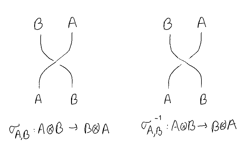
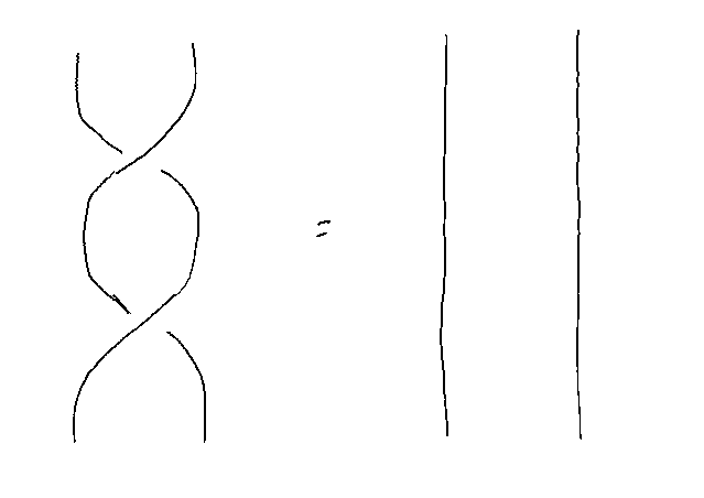
and the fact that \(\sigma_{A,B}\) admits an inverse for all objects \(A\) and \(B\), can be represented diagrammatically as
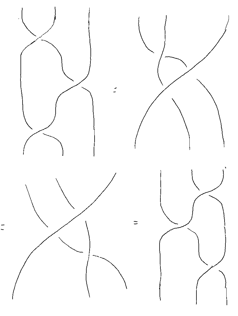
This captures the some part of the natural geometric behavior of strings in 3D space. Furthermore, naturality of the braiding implies that we can “drag ” morphisms along strings which are braided. Finally, the hexagon equations can also be represented graphically
Much like the simpler monoidal categories, braided monoidal categories also have a complete and sound graphical calculus with the inclusion of this braiding morphism, which can be stated as a theorem
Theorem (Correctness of the graphical calculus for braided monoidal categories):
A well-typed equation between morphisms in a braided monoidal category follows from the axioms if and only if it holds in the graphical language up to spatial isotopy.
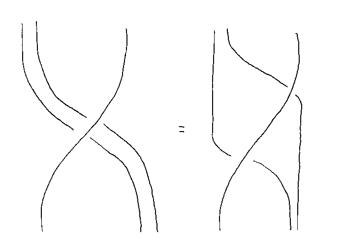
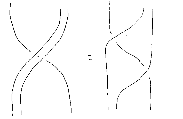
As an example, we can prove the so-called Yang-Baxter equation graphically for braided monoidal categories. The idea is to simply slide the braidings past each other in the following way
The simplest example of a braiding in a monoidal category, is the canonical braiding in Set , which is simply \(\sigma_{A,B}:A\times B\to B\times A\), which acts by sending \(\left(a,b\right)\mapsto\left(b,a\right),\forall a\in A,b\in B\). Similarly canonical braidings can be defined for Rel and Hilb as well. In particular, all these braidings have an additional property called symmetry.
Definition (Symmetric Monoidal category):
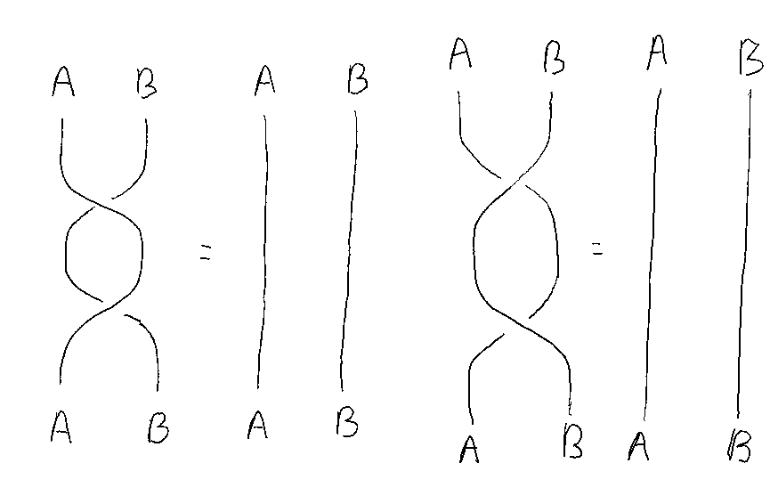
A monoidal category \(\boldsymbol{C}\)is symmetric when
\[\begin{equation} \sigma_{B,A}\circ\sigma_{A,B}=\text{id}_{A\otimes B}, \end{equation}\] for all objects \(A\) and \(B\) in \(\text{Ob}(\boldsymbol{C})\).
The braiding is often called the symmetry. Graphically, we can write this condition as
and furthermore, a symmetric monoidal category makes no distinction between “under-crossings ” and “over-crossings ”, which can be written as an equality
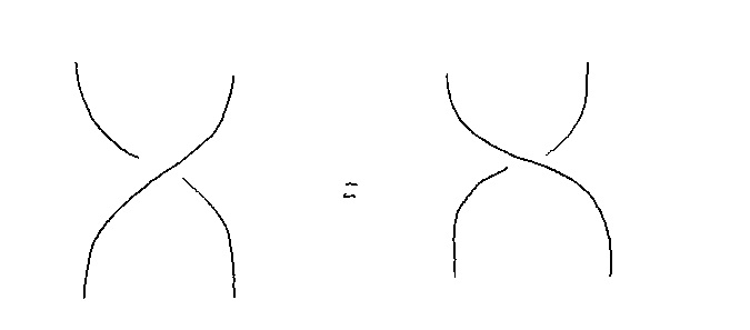
Thus, for symmetric monoidal categories, we can write the symmetry, correspondin g to the single type of crossing, as
For symmetric monoidal categories, one also has a notion of correctness of the graphical calculus, however, one has to mod out by the equality of over- and under-crossings. Stated as a theorem, this reads
Theorem (Correctness of the graphical calculus for symmetric monoidal categories ):
A well-typed equation between morphisms in a symmetric monoidal category follows from the axioms if and only if it holds in the graphical language up to graphical equivalence.
The part where I write “up to graphical equivalence means precisely this modding out by equivalence of braidings. Perhaps this can be formulated as isotopy in four dimensional space, this is not clear in the literature. An important example of symmetric monoidal categories, besides Set , Rel , and Hilb , and one which I most definitely return to in future posts is Rep ( G ). This is the group of finite-dimensional representations of a finite group G , in which
- Objects are finite-dimensional representations of G
- Morphisms are intertwiners for the group action
- The tensor product is the tensor product of representations
- The unit object is the trivial action of G on the one-dimensional vector space
- The symmetry is inherited from Vect
One of these days I may go into representation theory a bit deeper, and then I can cover these notions in more detail. For now, I leave them as open subjects to cover.
More to come
This has been a brief introduction to monoidal categories and diagrams. As per the previous post I have left out many examples of the famous categories , Set , Rel , and Hilb , which are usually studied in this context. I have also left out discussion about monoidal functors, strict categories, and the coherence theorem, which I will cover in the future, and have already written a bunch about. To avoid making this post longer, however, I will leave things here for now. I am thinking about making a post with a bunch of examples once I get the formal stuff out of the way.
One thing I also intend to do at some point is to make a series of posts about representation theory, of finite and Lie groups. This will be a large enterprise when I get to it, but one which I am looking forward to, and which will eventually trace back to categories, and specificall y, Rep ( G ). The idea is that I will someday get to use these things to talk about a categorical perspective of QFT and TQFT. Stay posted for all of that! Of course, before all of that I still have to talk about a bunch of stuff regarding categories, namely, about linear structure, and duality, to get to the main goal for now, which is introducing the necessary language for a categorical perspective on topologically ordered states.